TinyLoRA Explained: How 13 Parameters Taught an 8B Model to Reason

A paper from February 2026 does not usually resurface as the thing every AI researcher is texting each other about seven months later. But that is exactly what happened on September 16, 2026, when The Neuron's daily AI digest pulled "Learning to Reason in 13 Parameters" back into circulation, and within a day it was sitting near the top of Hacker News again [4]. The paper itself, by John X. Morris, Niloofar Mireshghallah, Mark Ibrahim, and Saeed Mahloujifar, was submitted to arXiv back on February 4, 2026 under the identifier 2602.04118 [1]. Nothing about it changed in the intervening months. What changed is that enough people finally sat with the number in the title and realized it is not a typo, a rounding error, or a narrow academic curiosity. It is a real, reproducible result, and it is strange enough that it is worth understanding properly instead of just retweeting the headline.

Here is the number, stated plainly, because it is worth pausing on before diving into the mechanism: researchers took Qwen2.5-7B-Instruct, an 8-billion-parameter language model, and improved its math reasoning accuracy using reinforcement learning while updating only 13 trainable parameters. Not 13 million. Not 13 thousand. Thirteen individual floating point numbers, stored in bfloat16, which comes out to 26 bytes total, smaller than a single AES-256 encryption key [1] [2]. With that 26-byte update, GSM8K accuracy moved from 88.2 percent to 91.8 percent [3] [4].

This post is a deep technical walkthrough of how that is possible: the truncated SVD trick that gives you a free basis of a weight matrix's most important directions, the fixed random projection that turns that basis into a single tunable knob, the weight tying that lets one tiny vector steer an entire model, and the specific property of reinforcement learning that makes any of this work at all. We will also cover where it breaks down, what the paper's authors themselves flag as unproven, and what it would actually take to try something like this on your own model. This is a genuinely technical post aimed at people who want to understand the mechanism, not just repeat the headline number, so expect real math, a runnable numpy demonstration, and worked comparisons against standard LoRA, LoRA-XS, and full fine-tuning.

Before we get into the steps, here is a video generation prompt that animates the same mechanism this post walks through, useful if you want to visualize the pipeline in motion rather than as a static diagram:

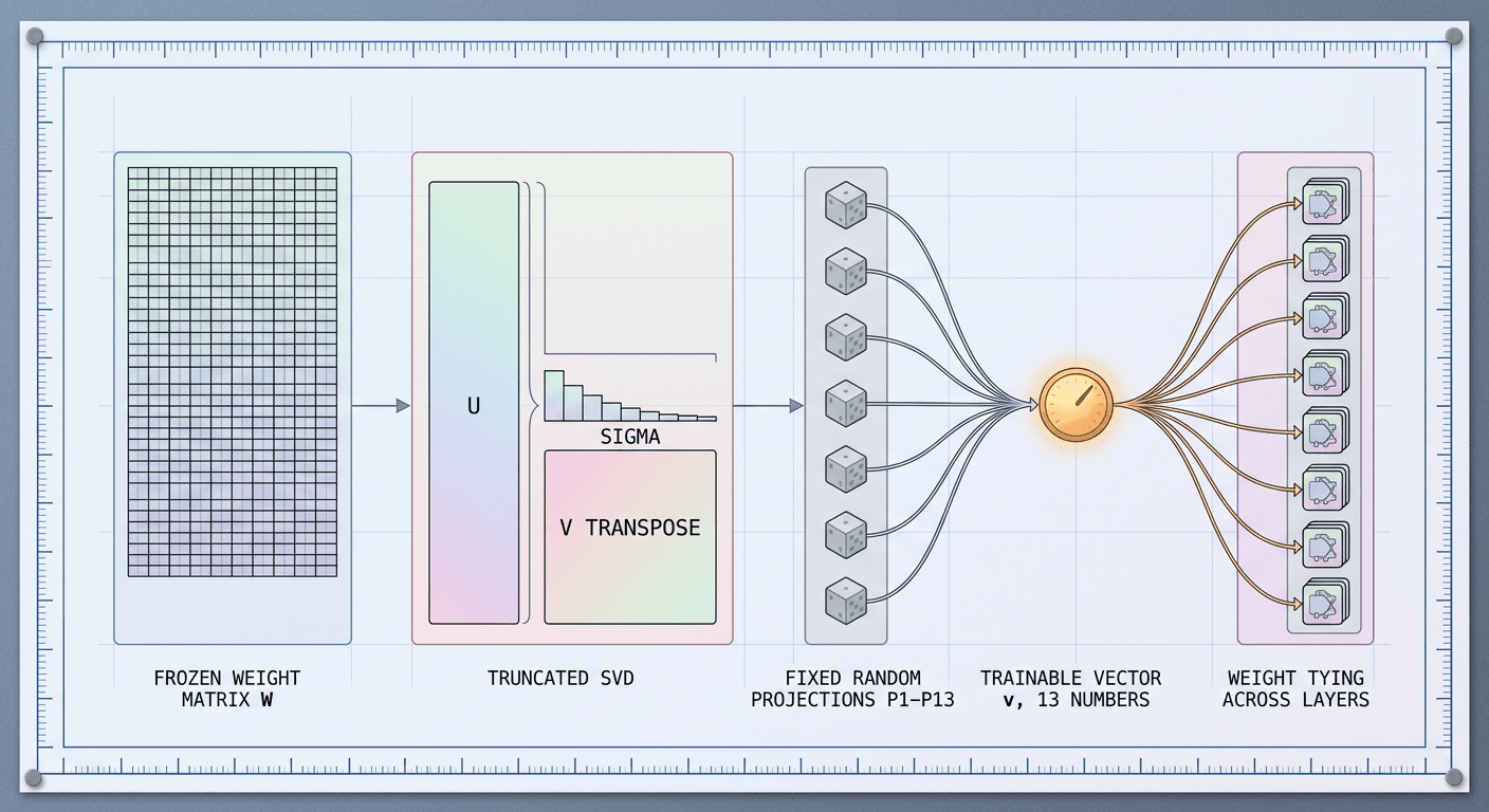
A Wan-style animated technical diagram video, pastel technical-blueprint line-art on a soft cream background with faint blueprint grid lines. Camera opens on a single labeled block reading 'FROZEN WEIGHT MATRIX W' rendered as a large rectangular grid of thin blue outlined cells. The block smoothly splits into three labeled sub-panels sliding apart left to right: 'U' (thin vertical bars), a diagonal gauge cluster labeled 'SIGMA, singular values sorted', and 'V TRANSPOSE' (thin horizontal bars), each captioned in short monospace-style text. Between U-Sigma and V-transpose, a small glowing amber node labeled 'v, 13 trainable numbers' pulses and sends thin animated lines into a bank of small frozen gray boxes labeled 'P1 through P13, fixed random tensors', each box lighting up briefly and feeding a weighted sum into a small matrix labeled 'R'. R slots into the gap, completing the equation 'W-prime equals W plus U Sigma R V-transpose' typeset in clean sans-serif along the bottom edge. The animation then pulls back to reveal the same amber 'v' node sending identical thin wires out to eight repeated copies of this same block, stacked vertically to represent transformer layers, each copy receiving the exact same 13-number signal while its own frozen random boxes differ slightly in shade to show they are independently sampled. Finally a small reward loop animates at the very bottom: a math problem icon feeds into the stacked layers, an output arrow splits into a green checkmark or red cross, and a thin animated arrow curves back up only to the amber 'v' node, visibly nudging its glow brighter or dimmer, while all the gray frozen boxes and the gridded W blocks stay completely static and untouched throughout. Smooth, even blueprint-style ambient lighting, thin ruler tick-mark border framing the whole scene, no photographic shading, no garbled text, every label short and legible, no logos or watermarks.

Step 1: Why "Rank-1" LoRA on an 8B Model Still Means Millions of Parameters

To appreciate why 13 parameters is startling, you first need to understand why standard low-rank adaptation, even pushed to its smallest conventional setting, still lands in the millions on a modern large language model.

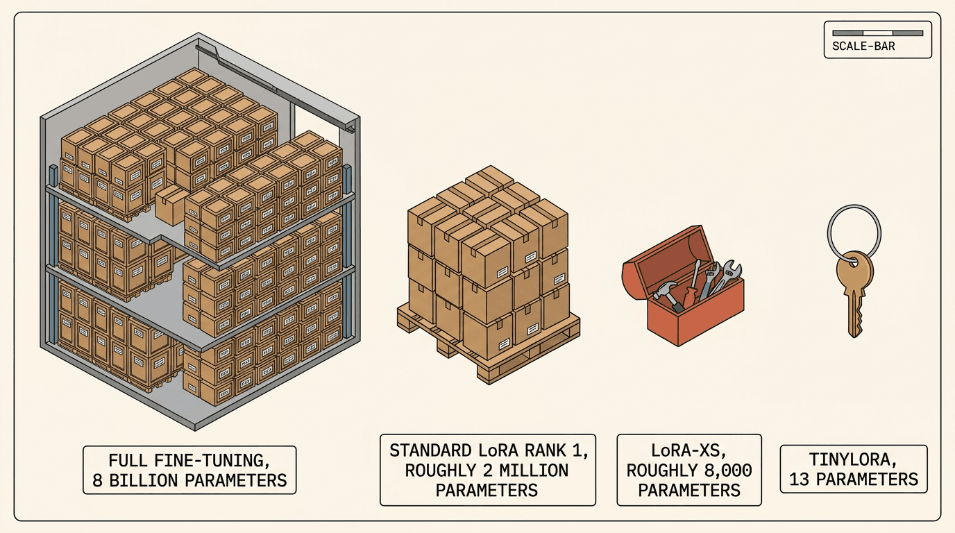
Standard LoRA, introduced by Hu et al. in 2021, freezes a pretrained weight matrix W and learns an additive update ΔW expressed as the product of two small matrices, A and B, so that the effective weight becomes W + BA [6]. If W is a d×d matrix, A is shaped r×d and B is shaped d×r, where r is the "rank" of the adapter. The trainable parameter count for that single matrix is 2dr. Set r to 1, the smallest rank anyone normally uses, and you still get 2d trainable parameters for that one matrix alone.

Here is where the "millions" comes from concretely. Take d = 4096, the hidden dimension used by several well-known 7-to-8B architectures such as Llama-2-7B and Llama-3-8B. A single rank-1 LoRA adapter on one d×d matrix costs 2 × 4096 = 8,192 parameters. That sounds almost small in isolation. The problem is that a transformer block does not have one d×d matrix, it has several: the query, key, value, and output projections inside attention, plus the up, down, and (in gated architectures) gate projections inside the MLP block. A typical 7-to-8B model has on the order of 28 to 32 transformer blocks. If you apply rank-1 LoRA to even just the four attention projections in every block, that is roughly 30 blocks × 4 matrices × 8,192 parameters ≈ 983,000 parameters, and if you extend it to the MLP projections too (which most practical LoRA recipes do, because attention-only adaptation tends to underperform), you are well past a million and climbing toward two or three million depending on exactly which matrices get adapted and whether K/V get folded through grouped-query attention's smaller shared projections.

That is the baseline every serious LoRA practitioner already accepts as "small." Millions of trainable parameters, versus the 8 billion in the full model, is already a roughly 3,000-to-1 compression ratio, and it is genuinely useful: it is why LoRA fine-tuning became the default way to specialize open models without needing a cluster. But millions is nowhere close to 13. Getting from "millions" to "single digits" is not a matter of turning a dial further in the same direction, shrinking r below 1 is not meaningful in the standard LoRA formulation, because A and B are dense, freely trainable matrices with no structure to exploit further. You need a fundamentally different parameterization, and that is where truncated SVD comes in.

Step 2: Truncated SVD Gives You a Basis of "Top Directions" for Free

Every real-valued matrix W has a singular value decomposition: W = UΣVᵀ, where U and V are orthogonal matrices whose columns are the left and right singular vectors, and Σ is a diagonal matrix of singular values sorted from largest to smallest. The singular vectors associated with the largest singular values capture the directions in which W has the most "energy," the directions a small perturbation would move the most output signal through. Truncating this decomposition to the top k singular vectors, keeping only the first k columns of U and V and the top-left k×k block of Σ, gives you the best possible rank-k approximation of W in the least-squares sense, a fact guaranteed by the Eckart-Young theorem.

This matters for parameter-efficient fine-tuning for a specific reason: instead of learning A and B from scratch as LoRA does, you can compute U, Σ, and V once, offline, directly from the already-trained weight matrix W, with zero gradient steps and zero trainable parameters. You get a ready-made, meaningful low-rank basis for free, just by running SVD on weights the model already has. This is exactly the idea behind LoRA-XS, published by Bałazy, Banaei, Aberer, and Tabor: freeze U and V from a truncated SVD of W, and insert one small trainable matrix R of shape r×r between them, so the update becomes W + UᵣRVᵣᵀ [7]. Because R is only r×r rather than the 2dr of standard LoRA, LoRA-XS reduces trainable parameters and storage by over 100x on 7B-scale models while matching or beating LoRA's accuracy on GLUE, GSM8K, MATH, and commonsense reasoning benchmarks [7].

Walk the parameter math through concretely. At rank r = 6, a LoRA-XS module needs r² = 36 trainable parameters, all inside R, compared to a standard rank-6 LoRA module's 2dr = 2 × 4096 × 6 = 49,152 parameters for the same matrix. That is already a roughly 1,365x reduction for that one module. Multiply 36 parameters by the roughly 200-plus modules across a full 8B model's attention and MLP layers, and you land somewhere around 7,000 to 9,000 trainable parameters for the whole model, orders of magnitude below standard LoRA, but still hundreds of times larger than TinyLoRA's headline 13. LoRA-XS proves that a frozen, SVD-derived basis is enough structure to fine-tune well with drastically fewer parameters. TinyLoRA's contribution is showing you can go much further than that, by changing what sits inside the gap between UΣ and Vᵀ.

Step 3: The Fixed Random Projection Trick

This is where TinyLoRA's actual mechanism lives, and it is worth writing the formula out in full before explaining each piece:

W' = W + UΣ(Σ_{i=1}^{u} v_i P_i)Vᵀ

Read from the outside in. U, Σ, and V come from a truncated SVD of the original frozen weight matrix W, exactly as in Step 2, computed once and never touched by gradient descent. The part that changes from LoRA-XS is what sits in the middle, where LoRA-XS had a freely trainable r×r matrix R, TinyLoRA has Σ_{i=1}^{u} v_i P_i, a weighted sum of u fixed random tensors P_1 through P_u, each one shaped to match R's slot, each one sampled once at initialization from a random distribution and then frozen forever. The only quantities that ever receive a gradient update are the u scalar weights v_1 through v_u, collected into a small vector v ∈ Rᵘ.

This is the crucial reframing. Instead of learning an r×r matrix directly, which has r² independent degrees of freedom, TinyLoRA fixes a small basis of u random r×r matrices ahead of time and learns only how much of each one to mix in. The model is not learning "what shape should the correction take," it is learning "how far along each of u pre-chosen fixed directions should I move." This is directly analogous to a classic dimensionality-reduction idea called random projection, well established in machine learning: a random linear map from a high-dimensional space to a much lower-dimensional one approximately preserves the geometric structure that matters, provided the lower dimension is large enough relative to the complexity of what you are trying to represent, a result formalized by the Johnson-Lindenstrauss lemma. TinyLoRA is applying that same intuition to the LoRA-XS recombination matrix itself: you do not need to learn the whole r×r space, you need to learn how to combine a handful of random directions inside it, because reinforcement learning's target update turns out to live in a very low-dimensional subspace to begin with.

Concretely, if u = 13 and each P_i is an r×r matrix with r = 6, that is 13 fixed 36-number random matrices (468 fixed, untrained numbers) sitting in a lookup table, and the entire trainable state of the model is the 13-number vector v that says how to blend them. Every one of the 468 numbers inside the P_i tensors is frozen; only the 13 coefficients ever move. This is why the parameter count for a single module drops from LoRA-XS's r² = 36 down to just u, which can be pushed as low as u = 1 for a single module in the paper's most extreme configurations, before weight tying is even applied. Weight tying is the next step, and it is what turns "13 trainable parameters per module" into "13 trainable parameters for the entire model."

python
/code
import numpy as np

rng = np.random.default_rng(42)

# --- Step 1: a toy frozen weight matrix (stand-in for one d x d module) ---
d = 64  # small stand-in for a real hidden dimension like 4096
r = 6   # truncated SVD rank kept
u = 13  # number of fixed random basis tensors / trainable scalars

W = rng.normal(scale=0.02, size=(d, d))

# --- Step 2: truncated SVD, computed once, frozen forever ---
U_full, S_full, Vt_full = np.linalg.svd(W)
U_r = U_full[:, :r]          # d x r, frozen
S_r = np.diag(S_full[:r])    # r x r, frozen
V_r = Vt_full[:r, :].T       # d x r, frozen

# --- Step 3: u fixed random r x r projection tensors, frozen forever ---
P = [rng.normal(scale=1.0, size=(r, r)) for _ in range(u)]

# --- Step 4: the ONLY trainable object, a length-u vector v, tied across modules ---
v = rng.normal(scale=0.01, size=u)

def recombination_matrix(v, P):
    # sum_{i=1}^{u} v_i * P_i -> an r x r matrix built from fixed randomness
    R = np.zeros_like(P[0])
    for vi, Pi in zip(v, P):
        R += vi * Pi
    return R

def tinylora_update(W, U_r, S_r, V_r, v, P):
    R = recombination_matrix(v, P)
    delta = U_r @ S_r @ R @ V_r.T
    return W + delta

W_prime = tinylora_update(W, U_r, S_r, V_r, v, P)

trainable_params = v.size
frozen_params = U_r.size + S_r.size + V_r.size + sum(p.size for p in P)

print(f"Toy module size: {d}x{d} = {d*d} weights")
print(f"Trainable parameters (v only): {trainable_params}")
print(f"Frozen SVD + random-projection parameters: {frozen_params}")
print(f"Frobenius norm of the update ||W' - W||: {np.linalg.norm(W_prime - W):.6f}")

# --- Weight tying demo: reuse the SAME v across a second, independent module ---
W2 = rng.normal(scale=0.02, size=(d, d))
U2, S2, Vt2 = np.linalg.svd(W2)
U2_r, S2_r, V2_r = U2[:, :r], np.diag(S2[:r]), Vt2[:r, :].T
P2 = [rng.normal(scale=1.0, size=(r, r)) for _ in range(u)]  # module-specific randomness
W2_prime = tinylora_update(W2, U2_r, S2_r, V2_r, v, P2)  # same v, different P

print(f"\nSame {u}-number vector v steers a second, unrelated module.")
print(f"Total trainable parameters across BOTH modules (tied): {v.size}")
print(f"Total trainable parameters WITHOUT tying would have been: {v.size * 2}")

Step 4: Weight Tying — One Shared Vector Steers Every Layer

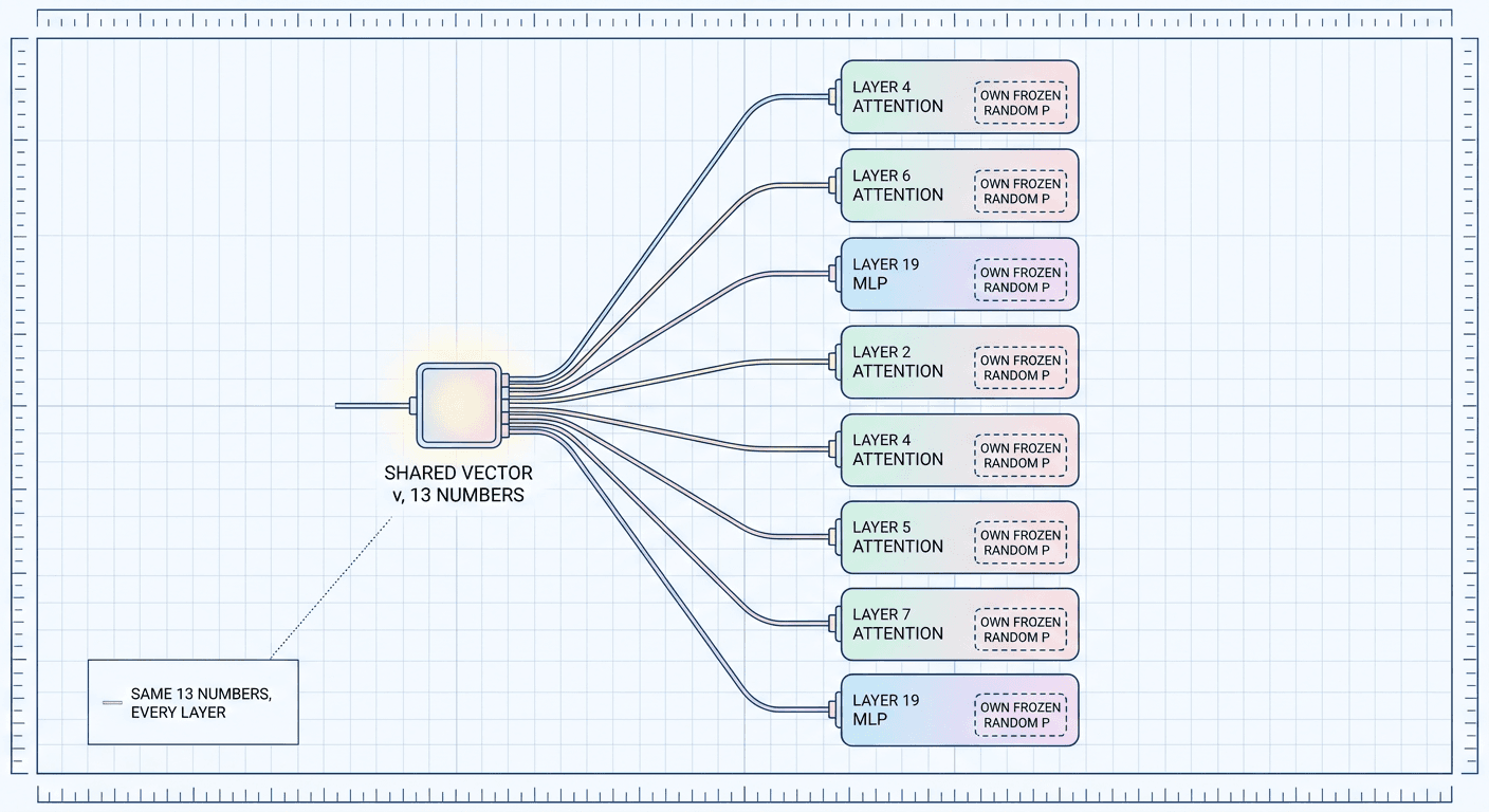
Even at u = 1 per module, a model with 200-plus adapted modules would still need 200-plus trainable parameters if every module learned its own independent v. Weight tying is the step that collapses that down to a genuinely global 13. The idea is to force every adapted module across the entire model, every attention projection in every transformer block, every MLP projection in every transformer block, to share the exact same trainable vector v. The fixed random tensors P_i are still sampled independently per module (there is no cost to that, since they are never trained and never even need to be stored if you can regenerate them from a fixed random seed), but the small number of scalars that actually receive gradients, the 13 entries of v, are the same 13 numbers everywhere in the network.

This is a strong, almost aggressive form of parameter sharing, and it is worth being honest about what it gives up. A single shared vector cannot express "increase this direction in layer 3's attention but decrease it in layer 20's MLP" independently, because the coefficients are identical everywhere; only the module-specific random tensor P_i differs, which changes how that shared blend gets expressed in each module's own SVD basis, but the blend weights themselves are locked together. What weight tying is betting on, and what the results show actually holds for math reasoning tasks, is that the useful update reinforcement learning wants to make is coherent enough across the model that a single low-dimensional "steering signal," reinterpreted through each layer's own local geometry via its own frozen U, Σ, V and its own frozen random P_i tensors, is enough to capture most of the benefit. Each layer effectively asks the same 13-number signal "what do you want from me," and answers it differently only because each layer's frozen SVD basis and random projections translate that identical signal into a different actual weight change.

This tying trick is also precisely what separates TinyLoRA from LoRA-XS in the comparison table worth keeping in your head: LoRA-XS ties the frozen SVD basis choice conceptually across the model (every module gets its own SVD-derived U, Σ, V) but still learns an independent r×r recombination matrix per module. TinyLoRA takes that one step further and ties the trainable recombination coefficients themselves across every module, using module-specific randomness instead of module-specific learning to do the differentiation. That single design choice is most of the distance between LoRA-XS's hundreds or thousands of trainable parameters and TinyLoRA's single digits.

Step 5: The RL Training Setup — Why GRPO's Reward Signal Is the Part That Makes This Work

TinyLoRA is trained with reinforcement learning, specifically a variant built around Group Relative Policy Optimization, or GRPO, the algorithm introduced in the DeepSeekMath paper and later popularized further through DeepSeek-R1 [8]. GRPO works by sampling a group of candidate completions for the same prompt, scoring each one with a reward function, and using the relative ranking within that group as the training signal, rather than training a separate learned critic network the way classic PPO does. For math reasoning tasks with automatically checkable answers, the reward function is about as simple as reward functions get: did the final answer match the ground truth, yes or no.

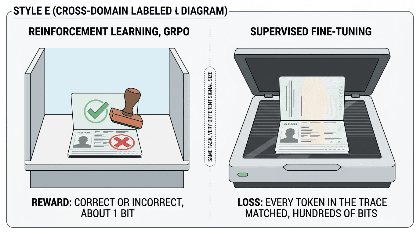
That single design choice, a binary, verifiable, sparse reward, is the real reason TinyLoRA's extreme compression is possible at all, and it is worth being precise about why. A reward signal that only says "right" or "wrong" per full generated solution carries, in an information-theoretic sense, at most one bit of information per training example, regardless of how long or complex the generated reasoning trace was to produce it. The optimization problem GRPO is actually solving, at this scale, reduces to nudging the model's existing latent reasoning behavior slightly more often toward "produces a correct final answer" and slightly less often toward "produces an incorrect one." That is a remarkably low-dimensional target. It does not require rewriting how the model reasons, expresses itself, or formats its output, it requires very slightly reweighting which of the reasoning paths the model already knows how to produce get sampled more often. A signal that thin can, it turns out, be steered by an update with almost no capacity of its own, because nearly all of the actual reasoning capability was already present in the frozen 8-billion-parameter base model. TinyLoRA is not teaching Qwen2.5 to reason, it is finding a tiny nudge that shifts an already-reasoning-capable model's sampling distribution toward its own better answers more consistently.

python
/code
import math

# A crude but concrete illustration of why a binary RL reward carries
# far less information per training example than a dense SFT loss.

def bits_for_binary_reward(p_correct=0.5):
    # One correct/incorrect outcome: at most 1 bit of information,
    # and less than 1 bit whenever the outcome is not a 50/50 coin flip.
    if p_correct in (0.0, 1.0):
        return 0.0
    return -(p_correct * math.log2(p_correct) + (1 - p_correct) * math.log2(1 - p_correct))

def bits_for_sft_trace(vocab_size=32000, trace_length=220):
    # Matching a specific token at a specific position, if the model
    # were choosing uniformly at random among the vocabulary, costs
    # log2(vocab_size) bits per position. Real models are far from
    # uniform, so treat this as an upper bound on the information a
    # full trace COULD carry, not a measured value.
    return trace_length * math.log2(vocab_size)

rl_bits = bits_for_binary_reward(p_correct=0.6)
sft_bits_upper_bound = bits_for_sft_trace()

print(f"RL reward information content (per completion): {rl_bits:.3f} bits")
print(f"SFT trace information upper bound (per completion): {sft_bits_upper_bound:,.1f} bits")
print(f"Ratio: SFT trace carries up to {sft_bits_upper_bound / rl_bits:,.0f}x more "
      f"information per training example than the binary RL reward.")
print()
print("This is the same order of magnitude as the paper's reported ~100-1000x")
print("gap in trainable parameters needed for SFT vs RL at these tiny budgets.")

Contrast this with what a dense, per-token reward or loss signal would demand, which is exactly the subject of Step 7 below on why supervised fine-tuning cannot be compressed this far. For now, the core training loop to have in mind: sample a batch of math problems, generate a group of candidate completions per problem with the current policy (base model plus the current 13-number v), score each completion's final answer as correct or incorrect, compute a GRPO-style relative advantage within each group, and backpropagate that advantage through the frozen U, Σ, V, and P_i tensors into gradients on the 13 numbers in v alone. Every other parameter in the 8-billion-parameter model, all 8 billion of them, stays completely frozen throughout training. Only those 13 floats move.

Step 6: The Benchmark Results in Detail

The headline GSM8K number, 88.2 percent baseline accuracy rising to 91.8 percent with the 13-parameter TinyLoRA adapter, is a 3.6 percentage point absolute gain [3] [4]. GSM8K is grade-school-level word problem math, so the baseline is already fairly strong, and closing roughly 30 percent of the remaining gap to perfect accuracy with a 26-byte update is the number that made the paper's title make sense to skeptical readers on first read.

The harder benchmarks tell a more interesting story, because they show the effect holding up, and in relative terms getting larger, as the underlying task gets harder. MATH500, a 500-problem benchmark spanning competition-level mathematics, moved from 64.6 percent to 74.6 percent, a full 10 percentage point absolute gain. AIME24, based on the American Invitational Mathematics Examination, a genuinely difficult competition math benchmark most models still struggle with, moved from 3.3 percent to 16.0 percent, which is not a modest bump, it is roughly a 4.8x relative improvement in accuracy from a 26-byte update. AMC23, based on the American Mathematics Competitions, moved from 30.0 percent to 54.5 percent, an 81.7 percent relative improvement [3]. Averaged across a six-benchmark suite the authors report, mean accuracy rose from 40.3 percent to 50.1 percent [4].

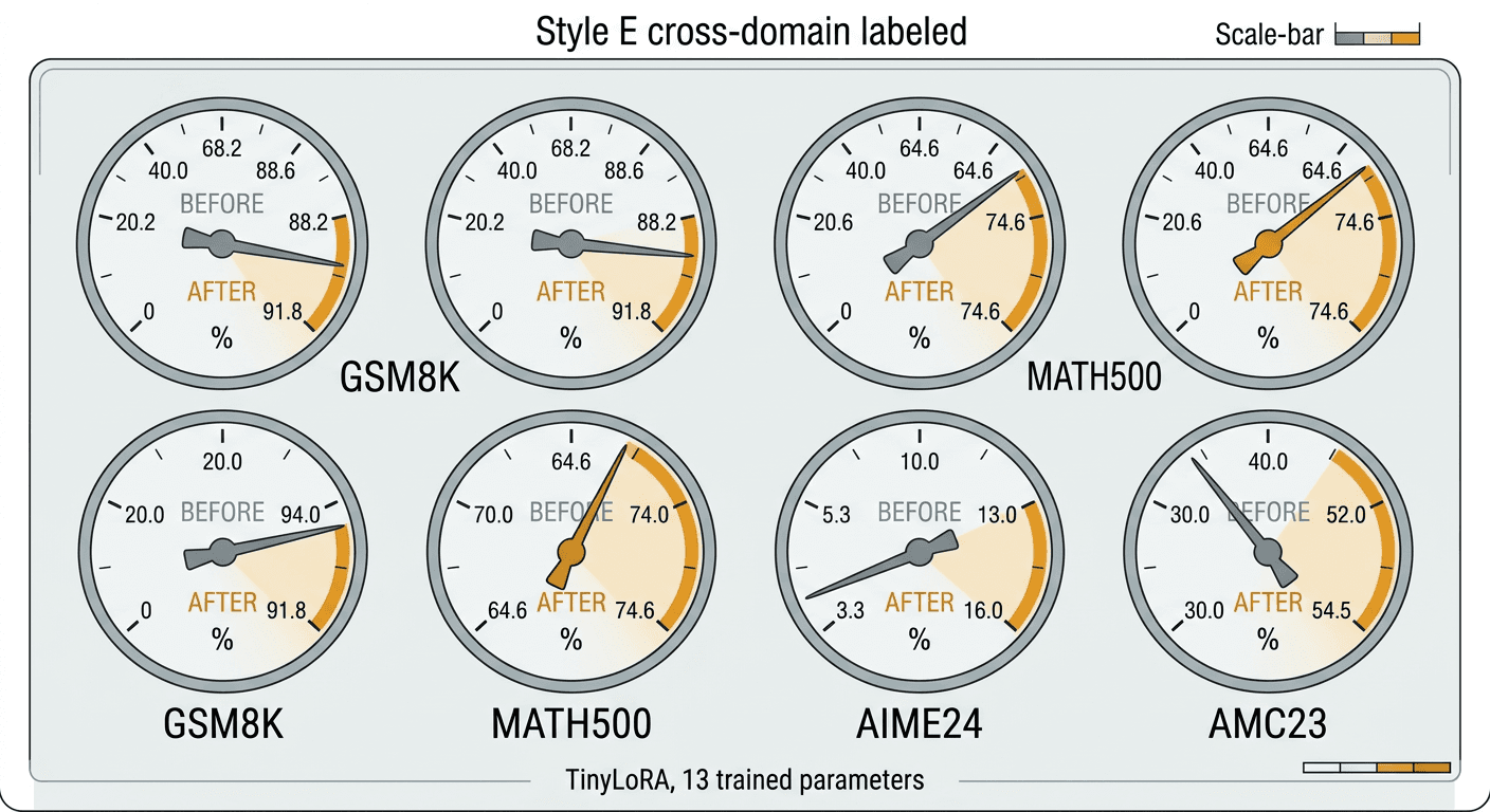
The comparison that matters most for judging whether this is a genuinely useful result, rather than a curiosity, is against full fine-tuning of the same model on the same task. Across these benchmarks, the 13-parameter (or near-minimal) TinyLoRA configuration recovers roughly 90 percent of the performance improvement that updating all 8 billion parameters achieves, while training on the order of 1,000 times fewer parameters than even a modest standard LoRA setup would need, and many orders of magnitude fewer than full fine-tuning [1] [2]. Put in a form that is easier to hold in your head: if full fine-tuning is worth 10 points of improvement on a given benchmark, TinyLoRA's 13-parameter update typically captures about 9 of those 10 points, using an update small enough to fit, with room to spare, in the space allotted for a single tweet's worth of text.

It's worth being precise that "13 parameters" describes the single most extreme configuration the paper reports, the one that makes for the best headline. The paper also reports configurations using up to roughly 200 trainable parameters, still an almost absurdly small number relative to 8 billion, and notes that these slightly larger budgets retain around 87 percent of full fine-tuning's absolute performance improvement across the harder MATH500, AIME, and AMC benchmarks specifically, a marginal improvement over the very smallest configuration at a cost of maybe an order of magnitude more parameters, still nowhere close to LoRA-XS's or standard LoRA's territory [2]. The overall shape of the result is consistent whether you look at the most extreme 13-parameter point or the slightly more generous 200-parameter point: both sit far below anything previously considered a "small" adapter, and both capture the large majority of what full fine-tuning buys you.

Step 7: Why Supervised Fine-Tuning Fails at This Scale

The single most important experimental finding in the paper, arguably more important than the 13-parameter headline itself, is that this entire approach only works when the training signal comes from reinforcement learning. Supervised fine-tuning on the exact same architecture, the exact same frozen SVD basis, the exact same fixed random projections and weight tying, needs roughly 100 to 1,000 times more trainable parameters than RL does to reach comparable accuracy [1] [2].

The explanation traces directly back to the information content of the two training signals, the same idea introduced in Step 5 but worth developing fully here because it is the paper's real thesis. GRPO's reward is a single bit per completion: correct or incorrect. Supervised fine-tuning, by contrast, provides a full token-by-token loss across an entire reasoning trace, typically hundreds of tokens for a nontrivial math problem, and the model is being asked to match that specific sequence of tokens as closely as possible, not just eventually land on the right final number. That per-token loss mixes together two very different kinds of information: the essential logical content of the solution (which step follows from which, which operation to apply next) and incidental surface detail that has nothing to do with correctness (exact phrasing, variable naming choices, which of several equally valid solution paths the reference trace happens to follow, whitespace and formatting conventions). A model being supervised-fine-tuned on that trace has to allocate capacity to match all of it, because the loss penalizes deviation from the reference sequence regardless of whether that deviation matters for correctness.

An update with only 13 or 200 degrees of freedom simply does not have room to encode "match this specific token sequence, including its incidental stylistic choices, across hundreds of positions." It has plenty of room to encode "nudge the sampling distribution slightly toward paths that happen to end correctly," because that is a much lower-dimensional target that does not care which correct path the model takes, only that it takes one. This is the same distinction that shows up more broadly in 2026's reinforcement-learning-for-reasoning research: RL with verifiable, sparse rewards has repeatedly proven to need far less capacity and far less carefully curated data than SFT to move a model's behavior in the intended direction, precisely because the reward is cheap to satisfy in many different ways rather than demanding exact sequence matching. TinyLoRA is, in a sense, an extreme stress test of that broader finding, pushed all the way down to see exactly how little capacity RL's sparse signal actually needs, and the answer turned out to be smaller than almost anyone had reason to guess going in.

There is a useful intuition pump for engineers who have not spent time with RL fine-tuning directly. Imagine teaching someone to solve a maze by only ever telling them, after they finish, whether they reached the exit or not, versus teaching them by handing them a fully annotated map of one specific correct path through the maze and grading them on how closely they retraced every turn. The first kind of feedback, the RL kind, lets the learner use whatever strategy they already have and just reinforces the parts of it that happen to work, which can be encoded in very few adjustable "preferences." The second kind, the SFT kind, demands the learner reproduce a specific path in detail, which requires memorizing far more information because there are many ways to solve a maze and only the annotated one is being rewarded during training.

Step 8: Architecture Dependence — Qwen2.5 vs Llama-3, and What's Still Unproven

Two honest limitations are worth taking as seriously as the headline result, and both come directly from the paper and its early technical coverage rather than from speculation.

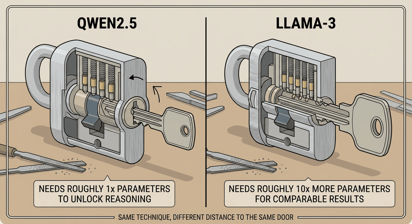
The first is architecture dependence. Reporting from Benjamin Marie's Kaitchup analysis notes that Qwen2.5 models need roughly 10 times fewer updated parameters than Llama-3 models to reach comparable performance under the same TinyLoRA setup [3]. The authors are upfront that they do not fully know why, whether it traces to differences in pretraining data mixture, differences in the post-training recipe each model family already went through before this experiment (Qwen2.5's own instruction-tuning and RLHF pipeline versus Llama-3's), or something about the geometry of the weight matrices themselves that makes certain SVD directions more directly aligned with "reasoning-relevant" behavior in one architecture than another. The practical reading of this finding is not "TinyLoRA doesn't work on Llama-3," the effect clearly still shows up, it is "the exact parameter budget you need is not a universal constant, it is a property of how close the base model's pretraining already left it to the desired reasoning behavior." A model that is already closer to reasoning well, in some latent sense, needs a smaller nudge to get there reliably. This reframes what RL fine-tuning at these tiny scales is actually doing: not injecting new capability, but unlocking or amplifying a direction that mostly already exists somewhere in the frozen weights, and some base models apparently sit closer to that direction than others.

The second limitation is scope, and it is the one the authors themselves flag most explicitly. Every strong result in the paper is demonstrated on math-style reasoning tasks with automatically verifiable rewards, problems where a script can check the final answer against a known correct value with no ambiguity. Whether this extreme compression holds up on open-ended, non-verifiable domains, creative writing quality, subjective helpfulness, code review judgment, multi-turn dialogue coherence, anything where "correct" is not a clean binary check, is explicitly untested and left as an open question [1]. This matters because the entire mechanistic explanation in Step 7 leans on the reward being a clean single bit of information. Non-verifiable domains typically use reward models or human preference signals that are noisier and higher-dimensional than "right or wrong," and it is a genuinely open empirical question whether that noisier signal still compresses down to single digits of trainable capacity, or whether it needs something closer to LoRA-XS's hundreds of parameters, or standard LoRA's millions, to capture reliably. Until someone runs that experiment and publishes the result, the honest summary is "extreme compression is proven for verifiable math reasoning, and unproven everywhere else," not "extreme compression is proven for RL fine-tuning in general."

What This Means for Real Tools and Practitioners

The practical relevance of this result is less about anyone actually shipping a 13-parameter production adapter tomorrow, and more about what it says regarding where the real bottleneck sits in parameter-efficient fine-tuning today.

The current ecosystem of PEFT methods already spans a wide range of tradeoffs. Standard LoRA remains the default in Hugging Face's own PEFT library because dense A and B matrices are simple to implement, easy to merge back into the base weights for zero-latency inference, and well understood. DoRA (Weight-Decomposed Low-Rank Adaptation) decomposes weight updates into magnitude and direction components and has shown improved accuracy over vanilla LoRA at similar parameter counts on several benchmarks. VeRA (Vector-based Random Matrix Adaptation) shares frozen random matrices across layers similarly in spirit to TinyLoRA, learning only small per-layer scaling vectors, and already demonstrated that shared randomness plus small trainable scalars can match LoRA's accuracy at a fraction of its parameter count, a genuine conceptual predecessor to the tying trick TinyLoRA pushes further. Prefix tuning takes a different axis entirely, learning virtual tokens prepended to the input rather than modifying weights at all. TinyLoRA fits into this landscape less as a brand-new axis and more as the current extreme end of a trend that VeRA and LoRA-XS were already pointing toward: fixed structure plus a shrinking number of trainable scalars, taken about as far as it can currently go, and specifically shown to need RL rather than SFT to work at the very bottom of that range.

Where this genuinely matters for infrastructure is multi-tenant adapter serving. Systems like S-LoRA, from Sheng et al., were built specifically to serve thousands of concurrent LoRA adapters against one shared base model, using unified memory paging to keep adapter weights and KV cache tensors in the same pool, and demonstrated up to 4x higher throughput than naive HuggingFace PEFT or vLLM serving while increasing the number of adapters served concurrently by orders of magnitude [9]. The bottleneck those systems are optimized around is adapter storage and adapter-swap latency: how many distinct A/B matrix pairs can you keep resident, and how fast can you page a different customer's adapter onto the GPU between requests. A standard rank-8 LoRA adapter for a 7-8B model can run into the tens of megabytes once you account for every adapted module; a LoRA-XS adapter shrinks that into the hundreds of kilobytes or less; a TinyLoRA-style adapter, at 13 to 200 parameters, shrinks the trainable payload itself down to a few dozen bytes to a couple of kilobytes, though the fixed random projection tensors and the SVD bases still need to be available at serving time (they can be regenerated deterministically from a stored seed rather than transmitted, which is itself a meaningful serving optimization). For platforms serving many personalized or task-specific fine-tunes off one shared base model, research at this end of the parameter-efficiency spectrum is part of why the marginal cost of storing and swapping one more customer's adapter keeps shrinking. Tools like Miraflow AI's AI Image Generator (https://miraflow.ai/create-ai-image) already run on efficiently served, fine-tuned generation models under the hood, and extreme parameter-efficiency research like this is exactly the kind of work that keeps pushing the operational cost of serving many personalized models down over time, even when a specific platform is not running this specific technique.

Common Mistakes and Misconceptions

Assuming 13 parameters means the model learned to reason from nothing. It did not. The 8 billion frozen parameters already encode almost all of the actual reasoning capability, from pretraining and whatever instruction tuning the base checkpoint already went through. The 13-parameter update is closer to a very precise steering correction on top of capability that was already mostly there, not a from-scratch skill acquisition. Framing it as "reasoning learned in 13 parameters" without that context invites the wrong mental model, and a more accurate framing is "13 parameters were enough to redirect an already-capable model's sampling distribution toward the reasoning paths it already knew how to produce."

Assuming this generalizes to supervised fine-tuning automatically. The paper's own headline result is explicitly an RL-only phenomenon. Attempting to replicate a 13-parameter SFT adapter on a similar task, expecting similar accuracy, contradicts the paper's central finding directly. SFT at this scale needs 100 to 1,000 times more parameters, per the authors' own reported experiments [1].

Assuming the fixed random projections don't matter and can be swapped for anything. The random tensors P_i are not incidental scaffolding, they define the specific low-dimensional subspace of the LoRA-XS recombination matrix that the trainable vector v is allowed to move within. A different random seed produces a different subspace, and while the paper's results suggest the specific random draw is not overly sensitive (random projections of sufficient dimension tend to preserve enough structure regardless of exact draw, per the Johnson-Lindenstrauss intuition from Step 3), swapping them for a structured or learned basis changes the method into something closer to LoRA-XS again, with a correspondingly larger parameter count.

Assuming this transfers straight to non-math, non-verifiable tasks. This is explicitly the open question the authors leave unanswered, not a settled extension. Treating a 13-parameter budget as a safe default for, say, a customer-support chatbot fine-tune or a creative writing style adapter is not supported by anything demonstrated in the paper. Reward models for open-ended tasks are noisier and carry more information per training example than a binary correctness check, and there is no published evidence yet that the same extreme compression survives that shift.

Confusing "13 trainable parameters" with "13 parameters total for the adapter's footprint." The frozen random tensors P_i and the frozen SVD factors U, Σ, V still need to exist somewhere at inference time, whether stored explicitly or regenerated deterministically from a fixed seed and the original base weights. The 13-number figure describes what gets updated during training and what needs to be stored or transmitted per fine-tune if the base model, SVD decomposition, and random seed are already shared infrastructure, not the total compute or memory footprint of running the adapted model.

Production Best Practices: What It Would Actually Take to Try This Yourself

If you wanted to reproduce an extreme-low-rank RL adapter on your own model rather than just reading about one, here is the realistic shape of the project, in the order the decisions actually need to be made.

Start with task selection, and be honest about it. This entire approach depends on having a cheap, automatic, sufficiently sparse reward function, matching the RL-vs-SFT explanation in Step 7. Math problems with a checkable final answer are the easy case. Code generation with unit tests that pass or fail is another reasonable candidate. Anything requiring a learned reward model or human preference judgments is starting from a fundamentally different, noisier signal, and the parameter budget that worked for math reasoning is not a safe assumption there; expect to need substantially more trainable capacity, closer to LoRA-XS's or even standard LoRA's range, until someone publishes evidence otherwise.

Next, pick your base model with the architecture-dependence finding from Step 8 in mind. If Qwen2.5-family models genuinely need an order of magnitude fewer parameters than Llama-3-family models to hit comparable accuracy, that is not just an academic footnote, it directly changes how aggressively you can compress if serving cost is a hard constraint. Budget a real ablation across at least two model families if serving cost is a hard requirement, rather than assuming whatever ratio held for math reasoning on Qwen2.5 transfers directly to your model and task.

Then implement the mechanism in three concrete pieces, matching Steps 2 through 4: run truncated SVD once, offline, on each weight matrix you intend to adapt, at a modest rank (the paper's own range spans roughly r = 1 up to the low dozens depending on configuration); sample and freeze your P_i random tensors once per module, ideally from a fixed, documented seed so they are exactly reproducible without needing to store the tensors themselves; and implement weight tying explicitly, meaning your training loop needs exactly one small trainable vector v, shared across every adapted module's forward pass, not one per module. A common implementation mistake here is accidentally letting each module keep its own instance of v because of how many frameworks default to per-module parameter registration; you have to actively register a single shared parameter and reference it from every adapted module's forward hook.

Configure GRPO (or a comparable group-relative RL algorithm) with a genuinely binary or otherwise sparse reward, sample multiple completions per prompt to get a usable within-group baseline the way GRPO's advantage estimation requires, and expect training to need meaningfully more sampled completions per gradient step than a dense-signal method would, since a sparse, low-information reward needs more samples to produce a low-variance gradient estimate on so few trainable parameters. Track validation accuracy on held-out problems from the same distribution as your reward's verification logic, not just training-set reward, since with only 13 to 200 degrees of freedom, overfitting in the traditional high-capacity sense is a smaller risk than simply misjudging the training distribution's alignment with your real target distribution.

Finally, before treating a very small parameter budget as validated, run the comparison the paper itself ran: the same setup with SFT on comparable trajectory data, at several parameter budgets, to confirm you actually need RL's sparse signal to get away with your chosen budget rather than assuming it. Skipping that comparison and just assuming "small works because the paper said small works" is the single most common way this technique gets misapplied, since the paper's central finding is specifically about RL's compressibility, not about compression in general.

Frequently Asked Questions

Is TinyLoRA a new model or a fine-tuning technique? It is a fine-tuning technique, not a model. It was demonstrated on Qwen2.5-7B-Instruct, an existing 8-billion-parameter open model, and the paper does not introduce a new base architecture. The 8 billion base parameters stay completely frozen throughout; only the small trainable vector described in Steps 3 and 4 gets updated.

Why is this paper trending now if it came out in February 2026? It was picked back up in AI news circulation via The Neuron's September 16, 2026 daily AI digest, which resurfaced it to a wide audience seven months after its original arXiv submission, and it climbed back onto Hacker News shortly after [4]. This is a genuine case of a result being extreme enough to keep resurfacing on its own merits rather than a new release.

Does 13 parameters mean the adapter uses almost no compute or memory to run? No, and this is a common point of confusion. The frozen base model still requires the same 8 billion parameters worth of compute and memory at inference time. What shrinks to 13 numbers is specifically the trainable, per-task adapter payload, the part that would otherwise need to be stored or transmitted separately per fine-tuned task if the base model and frozen SVD/random-projection infrastructure are already shared.

Can I use TinyLoRA for tasks other than math? The paper's verified results cover math reasoning with automatically checkable answers specifically. The authors explicitly flag generalization to open-ended, non-verifiable domains as untested, so treat any claim that this compresses equally well for tasks like creative writing or open-domain chat as unverified until someone publishes that experiment.

How does TinyLoRA compare to LoRA-XS specifically? Both start from the same idea, a frozen SVD basis of the original weight matrix. LoRA-XS learns a full r×r recombination matrix per module, landing in the hundreds to low thousands of trainable parameters for a whole model [7]. TinyLoRA replaces that learned r×r matrix with a weighted mix of fixed random tensors, learning only the mixing weights, and then ties that same mixing vector across every module in the model, which is what gets the count down into the single digits to low hundreds.

Is this the same as quantizing a LoRA adapter down to fewer bits? No. Quantization reduces how many bits represent each existing parameter (going from fp32 to int8, for example) without changing how many parameters there are. TinyLoRA reduces the actual count of trainable parameters through structural reparameterization, truncated SVD plus fixed random projections plus weight tying, and then separately stores those few remaining parameters in an ordinary precision like bf16. The two techniques are complementary, not the same idea.

Why does reinforcement learning specifically enable this, and not just "better optimization"? It comes down to the information content of the training signal, covered in depth in Step 7. GRPO's reward is close to one bit per completion (correct or incorrect), which is cheap to encode into very few trainable parameters. Supervised fine-tuning's per-token loss carries far more information per example, including incidental stylistic detail unrelated to correctness, and needs proportionally more trainable capacity to absorb it, roughly 100 to 1,000 times more according to the paper's own reported comparison [1].

Conclusion

TinyLoRA is not a trick that makes fine-tuning universally cheaper. It is a precise, well-controlled demonstration of something more specific and, in its own way, more interesting: that reinforcement learning's sparse, verifiable reward signal can be compressed into an astonishingly small number of trainable parameters when the underlying base model already has most of the needed capability latent in its weights, and truncated SVD plus fixed random projections plus aggressive weight tying give you a principled way to find and exploit that low-dimensional steering direction. The mechanism traces cleanly through four real ideas: a free, structured basis from SVD, a fixed random subspace inside that basis, a single shared vector tied across the whole model, and a reward signal thin enough to fit inside that vector's tiny capacity. None of the four pieces is individually exotic; VeRA had already shown fixed random matrices plus small trainable vectors could work, LoRA-XS had already shown a frozen SVD basis was enough structure to fine-tune well, and GRPO's binary reward was already the standard for verifiable-reward RL. What TinyLoRA adds is combining all three at once and pushing the resulting parameter count all the way down to see where it actually breaks, and the honest answer the paper gives is that, for math reasoning specifically, it does not break until you are down to single digits.

The caveats matter as much as the headline. This is proven on verifiable math reasoning and explicitly unproven elsewhere, it depends on the base model already being close to reasoning well, and its parameter budget is architecture-dependent in ways the authors themselves cannot fully explain yet. Treat it as a genuinely useful data point about how little capacity RL fine-tuning needs under the right conditions, not as a universal recipe to copy onto the next unrelated fine-tuning project. For the broader engineering picture of where these efficiency gains actually land in production, research at this extreme end of parameter-efficient fine-tuning is part of the same trend line as multi-adapter serving systems like S-LoRA, and it is exactly the kind of work that keeps lowering the real cost of running many fine-tuned, personalized models off one shared base, the same economic pressure that shapes how platforms serving fine-tuned generation at scale, Miraflow AI's AI Image Generator (https://miraflow.ai/create-ai-image) among them, keep their own serving costs manageable as personalization demand grows.

References and Sources

[1] Morris, J.X., Mireshghallah, N., Ibrahim, M., Mahloujifar, S. "Learning to Reason in 13 Parameters." arXiv:2602.04118, submitted February 4, 2026.

[2] EmergentMind. "Learning to Reason in 13 Parameters (paper summary)."

[3] Marie, B. "LoRA, But With Only 13 Parameters." The Kaitchup.

[4] The Neuron. "Everything That Happened in AI Today (Wednesday, September 16, 2026)."

[5] MarkTechPost. "This AI Paper Introduces TinyLoRA, A 13-Parameter Fine-Tuning Method That Reaches 91.8 Percent GSM8K on Qwen2.5-7B."

[6] Hu, E.J., Shen, Y., Wallis, P., Allen-Zhu, Z., Li, Y., Wang, S., Wang, L., Chen, W. "LoRA: Low-Rank Adaptation of Large Language Models." arXiv:2106.09685.

[7] Bałazy, K., Banaei, M., Aberer, K., Tabor, J. "LoRA-XS: Low-Rank Adaptation with Extremely Small Number of Parameters." arXiv:2405.17604.

[8] Shao, Z., Wang, P., Zhu, Q., et al. "DeepSeekMath: Pushing the Limits of Mathematical Reasoning in Open Language Models." arXiv:2402.03300.

[9] Sheng, Y., Cao, S., Li, D., et al. "S-LoRA: Serving Thousands of Concurrent LoRA Adapters." arXiv:2311.03285.