Time Series Forecasting with Transformers: From Theory to Implementation

Introduction

Time-series data support critical functions in forecasting, anomaly detection, resource optimization, and real-time decision making across finance, healthcare, energy systems, and networked computing.[1] From predicting electricity consumption and stock prices to forecasting weather patterns and patient health trajectories, our ability to anticipate the future hinges on how well we model the past. For decades, classical statistical approaches like ARIMA and exponential smoothing served as the gold standard for time series forecasting, followed by deep learning models such as RNNs and LSTMs that brought nonlinear modeling capabilities to the table.

But these methods have an Achilles' heel. Classical statistical approaches and early deep-learning architectures (RNNs, LSTMs, CNNs) have achieved notable progress, yet they exhibit structural limitations: recurrent models struggle with long-range dependencies, convolutional models require deep stacking to enlarge receptive fields, and both scale suboptimally to high-dimensional and high-volume data.[1]

Enter the Transformer. Transformers have achieved superior performances in many tasks in natural language processing and computer vision, which also triggered great interest in the time series community. Among multiple advantages of Transformers, the ability to capture long-range dependencies and interactions is especially attractive for time series modeling, leading to exciting progress in various time series applications.[3]

This blog post takes you on a comprehensive journey from the foundational theory of how Transformers work on time series data, through the major architectural innovations that defined the field, all the way to practical implementation with modern frameworks and the latest frontier of time series foundation models.

Why Transformers for Time Series?

To understand why Transformers have become so compelling for time series, we need to appreciate what they bring that previous architectures couldn't.

RNNs and LSTMs process sequences step by step, maintaining a hidden state that supposedly carries information from earlier time steps to later ones. In practice, this sequential bottleneck means that information from 500 time steps ago has been compressed through hundreds of transformations, often degrading beyond usefulness. Gradient vanishing and explosion make training on long sequences fragile and slow.

The self-attentive mechanism of the Transformer allows for adaptive learning of short-term and long-term dependencies through pairwise (query-key) request interactions. This feature grants the Transformer a significant advantage in learning long-term dependencies on sequential data, enabling the creation of more robust and expansive models.[10]

The Transformer's self-attention mechanism computes relationships between every pair of time steps in parallel, meaning the model can directly attend to an event 500 steps ago with the same ease as attending to the previous step. This parallel computation also means training is dramatically faster on modern GPU hardware compared to the sequential nature of recurrent models.

However, this power comes at a cost: the standard self-attention mechanism has O(L^2) time and memory complexity, where L is the sequence length. However, there are several severe issues with Transformer that prevent it from being directly applicable to LSTF, including quadratic time complexity, high memory usage, and inherent limitation of the encoder-decoder architecture.[4] Much of the innovation in time series Transformers has been about taming this quadratic cost while preserving (or even improving) the model's ability to capture temporal patterns.

The Core Challenge: Time Series ≠ Language

Before diving into architectures, it's essential to understand why we can't simply take a language Transformer like GPT and apply it directly to time series. Time series data presents unique challenges that demand specialized adaptations.

First, there is the problem of continuous values versus discrete tokens. In NLP, the input is a sequence of discrete tokens from a finite vocabulary. Time series values are continuous and unbounded, requiring different embedding strategies. Second, time series exhibit multi-scale temporal patterns: daily cycles, weekly seasonality, annual trends, and irregular shocks all coexist in a single sequence. Third, multivariate dependencies mean that multiple variables (e.g., temperature, humidity, and wind speed) evolve together, and capturing their cross-variable relationships is critical. Finally, non-stationarity — the statistical properties of time series change over time — poses challenges that don't typically arise in language modeling.

However, genuine time-series data tends to be noisy and non-stationary, and learning spurious dependencies, lacking interpretability, can occur if time-series-related knowledge is not combined.[10]

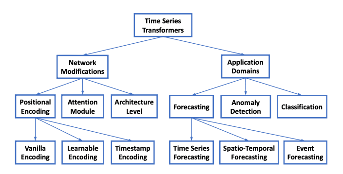
These challenges have spawned a rich taxonomy of approaches. From the perspective of network structure, we summarize the adaptations and modifications that have been made to Transformers in order to accommodate the challenges in time series analysis. From the perspective of applications, we categorize time series Transformers based on common tasks including forecasting, anomaly detection, and classification.[3]

The Mathematics: Self-Attention for Temporal Data

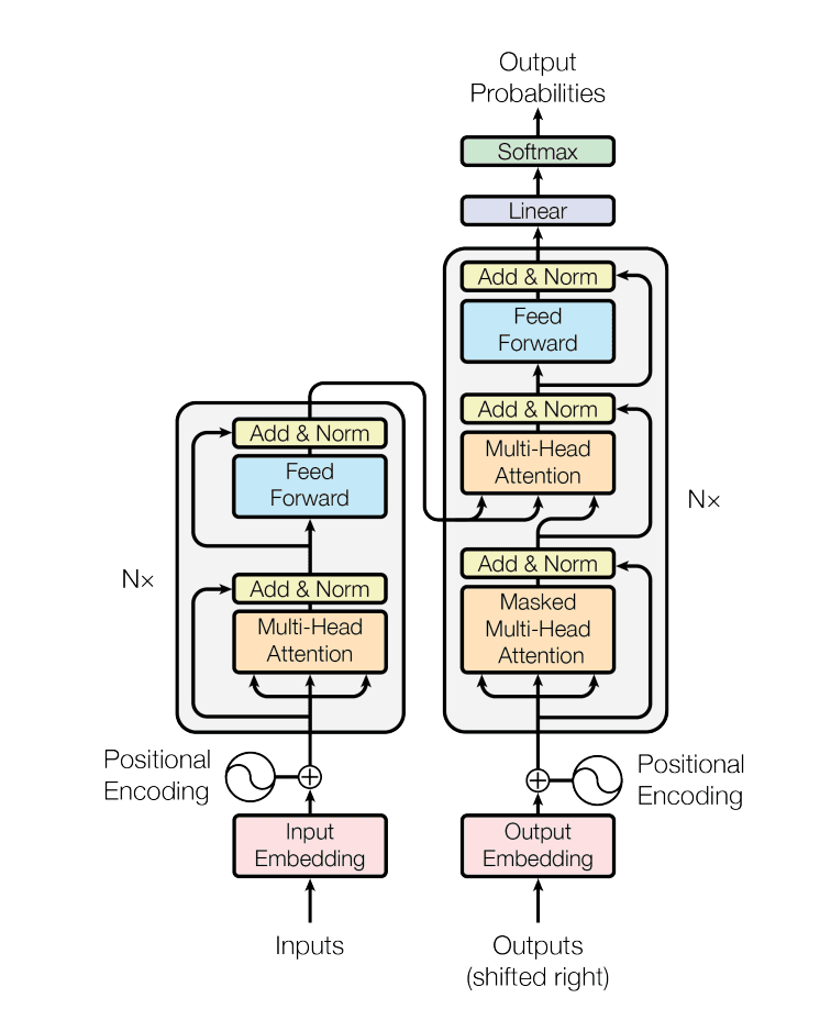
At the heart of every Transformer-based time series model lies the self-attention mechanism. Given an input sequence of time series values X∈R^L×d where L is the sequence length and ddd is the feature dimension, the model first projects the input into three representations — queries Q, keys K, and values V — through learned linear transformations:

The attention output is then computed as:

In the context of time series, this means every time step can attend to every other time step, weighted by their learned relevance.

Multi-head attention extends this by running hhh parallel attention operations with different projections, enabling the model to simultaneously capture different types of temporal relationships (e.g., one head might focus on short-term local patterns while another captures seasonal periodicity):

For time series, positional encoding takes on special significance. Unlike language where word order conveys syntactic meaning, the position in a time series conveys temporal information. Models typically use either sinusoidal encodings, learnable position embeddings, or specialized temporal embeddings that encode features like hour-of-day, day-of-week, or month-of-year directly.

The Tokenization Question: How to Feed Time Series to a Transformer

One of the most consequential design decisions in time series Transformers is how to convert the raw time series into tokens that the model processes. These models utilize different tokenization strategies, point-wise, patch-wise, and variate-wise, to represent time-series data, each resulting in different scope of attention maps.[2]

Point-wise tokenization treats each individual time step as a single token. This is the most straightforward approach and was used by early models like the vanilla Transformer and Informer. However, each token carries very little semantic information (just a single number), and the sequence length equals the number of time steps, leading to high computational cost.

Patch-wise tokenization segments the time series into contiguous patches of multiple time steps, analogous to how Vision Transformers (ViT) split images into patches. This is the approach championed by PatchTST and has become arguably the most influential design choice in recent years. Patching design naturally has three-fold benefit: local semantic information is retained in the embedding; computation and memory usage of the attention maps are quadratically reduced given the same look-back window; and the model can attend longer history.[2]

Variate-wise tokenization embeds the entire time series of each variable as a single token, as proposed by iTransformer. We propose iTransformer that simply applies the attention and feed-forward network on the inverted dimensions. Specifically, the time points of individual series are embedded into variate tokens which are utilized by the attention mechanism to capture multivariate correlations; meanwhile, the feed-forward network is applied for each variate token to learn nonlinear representations.[1]

An important recent finding is that despite the emergence of sophisticated architectures, simpler transformers consistently outperform their more complex counterparts in widely used benchmarks.[2] Research from ICML 2025 showed that most useful information comes from tracking patterns within individual variables over time, rather than between variables. Techniques like data normalization and skip connections also contribute significantly to forecasting performance.[2]

The Evolution of Time Series Transformers

The development of Transformer architectures for time series forecasting has proceeded through several distinct phases, each addressing limitations discovered in the previous generation.

Phase 1: Taming Quadratic Complexity — Informer (2021)

Many real-world applications require the prediction of long sequence time-series, such as electricity consumption planning. Long sequence time-series forecasting (LSTF) demands a high prediction capacity of the model, which is the ability to capture precise long-range dependency coupling between output and input efficiently.[4]

The Informer, which won the AAAI 2021 Best Paper award, was among the first to tackle the Transformer's scalability problem for long-horizon time series forecasting head-on. The architecture has three distinctive features: A ProbSparse self-attention mechanism with an O time and memory complexity Llog(L). A self-attention distilling process that prioritizes attention and efficiently handles long input sequences. An MLP multi-step decoder that predicts long time-series sequences in a single forward operation rather than step-by-step.[3]

The ProbSparse attention mechanism works by observing that in practice, the attention score distribution is often sparse, only a handful of queries actively attend to keys, while the rest produce near-uniform distributions. By measuring the "sparsity" of each query using KL-divergence from the uniform distribution, Informer selects only the top-u most active queries, reducing computation from O(L^2) to O(Llog⁡L). Among the first breakthroughs was Informer, which outperformed vanilla Transformers by 15–20% on datasets like ETT and Weather, while also speeding up training and inference.[1]

Phase 2: Decomposition Meets Attention — Autoformer (2021)

While Informer made major strides in handling long time series efficiently, it still treated time as just a sequence of numbers, every time step weighed the same, regardless of whether it was a peak, a seasonal dip, or a long-term trend. But real-world time series aren't flat, they have structure. For example, sales rise during holidays, electricity demand peaks in the evenings, and Mondays don't behave like Sundays.[1]

Autoformer builds upon the traditional method of decomposing time series into seasonality and trend-cycle components. This is achieved through the incorporation of a Decomposition Layer, which enhances the model's ability to capture these components accurately. Moreover, Autoformer introduces an innovative auto-correlation mechanism that replaces the standard self-attention used in the vanilla transformer. This mechanism enables the model to utilize period-based dependencies in the attention, thus improving the overall performance.[2]

The Auto-Correlation mechanism is a clever departure from standard attention. Instead of comparing individual time steps, it operates in the frequency domain to discover period-based dependencies, essentially finding which lagged copies of the series are most similar. Generally, for the long-term forecasting setting, Autoformer achieves SOTA, with a 38% relative improvement over previous baselines.[7] It was even deployed operationally during the 2022 Winter Olympics for weather forecasting at competition venues.

Phase 3: Frequency Domain Enhancement — FEDformer (2022)

FEDformer moves into the frequency domain, using Fourier transforms to isolate dominant patterns in the data, and it improves accuracy by over 22% on univariate tasks compared to Autoformer.[1]

The FEDformer algorithm model uses a decomposed encoder–decoder overall architecture such as the Autoformer algorithm model. To improve the efficiency of subsequence-level similarity computation, the FEDformer algorithm model uses methods such as Fourier analysis. In general, the Autoformer algorithm model can be said to decompose the sequence into multiple time-domain subsequences for feature extraction, whereas the FEDformer algorithm model uses frequency transform to decompose the sequence into multiple frequency domain modes for feature extraction.[8]

By operating directly on frequency components, FEDformer achieves linear computational complexity while capturing global temporal patterns. The key insight is that in the frequency domain, a small number of Fourier modes often capture most of the signal's energy, enabling aggressive compression without sacrificing important patterns.

Phase 4: The Patching Revolution — PatchTST (2023)

PatchTST, published at ICLR 2023, represents perhaps the most important paradigm shift in time series Transformers. Its title "A Time Series is Worth 64 Words" immediately signals the core idea: treating chunks of time series as analogous to word tokens. We propose an efficient design of Transformer-based models for multivariate time series forecasting and self-supervised representation learning. It is based on two key components: (i) segmentation of time series into subseries-level patches which are served as input tokens to Transformer; (ii) channel-independence where each channel contains a single univariate time series that shares the same embedding and Transformer weights across all the series.[2]

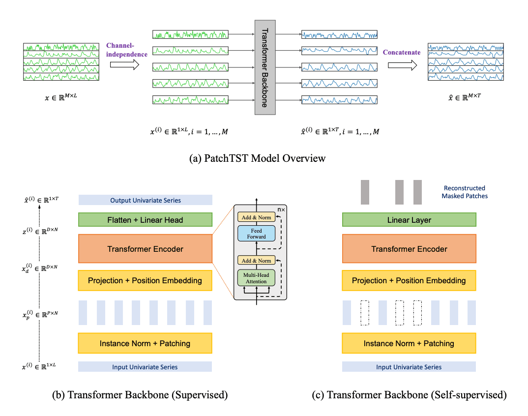
The channel-independence design is counterintuitive — why ignore cross-variable relationships? — but it works remarkably well in practice. While typical Transformer models mix features across channels, prior work with CNNs and linear models has shown that modeling univariate series separately can be more effective.[6] By sharing the same Transformer backbone across all channels, PatchTST achieves implicit regularization and avoids the overfitting that plagues models trying to learn cross-channel patterns from limited data.

Compared with the best results that Transformer-based models can offer, PatchTST/64 achieves an overall 21.0% reduction on MSE and 16.7% reduction on MAE, while PatchTST/42 attains an overall 20.2% reduction on MSE and 16.4% reduction on MAE.[4]

PatchTST also supports self-supervised pre-training via masked patch reconstruction, directly inspired by masked autoencoders in vision. In addition to supervised forecasting, PatchTST supports self-supervised pretraining via masked patch reconstruction, inspired by masked autoencoders in NLP and vision. The model uses non-overlapping patches to ensure that masked regions can be cleanly separated from observed ones. A subset of patches is selected uniformly at random and zero-masked.[6]

Phase 5: Inverting the Paradigm — iTransformer (2024)

iTransformer has been accepted as ICLR 2024 Spotlight.[2] While PatchTST proved the power of channel-independence, iTransformer took a radically different approach: what if we invert the entire Transformer architecture?

Based on the above motivations, we believe it is not that Transformer is ineffective for time series forecasting, but rather it is improperly used. In this paper, we revisit the structure of Transformer and advocate iTransformer as a fundamental backbone for time series forecasting.[5]

Considering the characteristics of multivariate time series, iTransformer breaks the conventional structure without modifying any Transformer modules. Inverted Transformer is all you need in MTSF.[2] The model embeds each variable's entire history into a single token, then uses attention across variable tokens to capture multivariate correlations, while the feed-forward network learns temporal representations within each variable.

While previous Transformers do not necessarily benefit from the increase of historical observation, iTransformers show a surprising improvement in forecasting performance with the increasing length of the lookback window.[8] This is a significant practical advantage: iTransformer can actually leverage longer histories, something vanilla Transformers notoriously fail to do.

The "Are Transformers Even Effective?" Debate

The field experienced a dramatic shake-up in 2023. In the paper Are Transformers Effective for Time Series Forecasting?, published recently in AAAI 2023, the authors claim that Transformers are not effective for time series forecasting. They compare the Transformer-based models against a simple linear model, which they call DLinear. The DLinear model uses the decomposition layer from the Autoformer model. The authors claim that the DLinear model outperforms the Transformer-based models in time-series forecasting.[2]

This paper sent shockwaves through the community, questioning whether all the architectural sophistication was justified when a single linear layer could outperform Informer, Autoformer, and FEDformer. The Transformer, introduced in 2017, was initially hailed as a definitive solution for time-series forecasting due to its ability to capture long-term dependencies in parallel. However, a report at AAAI 2023... Nevertheless, as of 2025, fundamental challenges remain, including the sharpness of the loss function and the interpretability of attention.[7]

However, subsequent work revealed that the comparison was not entirely fair. Our comparison shows that the simple linear model, known as DLinear, is not better than Transformers as claimed. When compared against equivalent sized models in the same setting as the linear models, the Transformer-based models perform better on the test set metrics we consider.[2] The models like PatchTST and iTransformer that emerged after this critique decisively demonstrated that Transformers are indeed effective, the issue was in how they were being applied, not in the architecture family itself.

Temporal Fusion Transformer (TFT): The Practitioner's Favorite

While models like PatchTST and iTransformer dominate academic benchmarks, the Temporal Fusion Transformer (TFT) holds a special place in practical deployments. While not always the most accurate in benchmarks, TFT is known for its practical strengths. It supports exogenous inputs, provides uncertainty estimates, and offers interpretability through attention visualization, traits that make it valuable in real-world deployment.[1]

TFT integrates several critical capabilities that production systems need. It supports three types of inputs: static metadata (e.g., store ID), known future inputs (e.g., holidays, planned promotions), and observed inputs (e.g., past sales). It uses variable selection networks to automatically determine which inputs are most relevant, gated residual networks for nonlinear processing, and interpretable multi-head attention that reveals which past time steps influenced the forecast most. Crucially, it produces quantile forecasts, giving not just a point prediction but a full distribution of possible outcomes.

The Foundation Model Era: Chronos, TimesFM, and Moirai

The latest and perhaps most transformative development in the field is the emergence of time series foundation models, large models pre-trained on massive corpora of time series data that can perform zero-shot forecasting on entirely unseen datasets. From late 2024 to early 2025, a wave of new time-series foundation models was released by major vendors like Amazon, Google, Salesforce, and others.[1]

Time Series Foundation Models (TSFMs) are an emerging class of time series forecasting models inspired by the architecture and training procedures of foundation models in natural language processing, especially Large Language Models (LLMs). Prominent examples of TSFMs include Chronos (Ansari et al., 2024), TimesFM (Das et al., 2024), Moirai/Moirai-MoE (Woo et al., 2024; Liu et al., 2024b), MOMENT (Goswami et al., 2024) and Time-MoE (Shi et al., 2024).[3]

Chronos (Amazon) takes an innovative approach by repurposing language model architectures. Chronos is technically a framework to repurpose a large language model (LLM) for time series forecasting developed by Amazon. The researchers have pretrained models based on the T5 family that can be used for zero-shot forecasting. The framework implies tokenizing time series data points, by scaling the data and performing quantization to create a fixed "vocabulary" of time, such that it can be used directly with LLMs.[4]

TimesFM (Google) is a decoder-only foundation model designed for point forecasting. TimesFM is decoder-based foundation model developed by Google Research. It is a deterministic model focusing on point forecasts. It relies on patching the series to extract local semantic information from groups of data points. The model patches the input series and is trained to output longer output patches, such that it undergoes less autoregressive steps if the forecast horizon exceeds the output patch length.[4]

Moirai (Salesforce) brings probabilistic forecasting to the foundation model paradigm. Moirai is an encoder-only transformer model developed by Salesforce. It is a probabilistic model that also relies on patching the input series. It supports both historical and future exogenous variables. A distinct feature of Moirai is that it uses a mixture distribution, using four different distributions, to output more flexible prediction intervals.[4]

Time series forecasting is undergoing a transformative shift. The traditional approach of developing separate models for each dataset is being replaced by the concept of universal forecasting, where a pre-trained foundation model can be applied across diverse downstream tasks in a zero-shot manner, regardless of variations in domain, frequency, dimensionality, context, or prediction length. This new paradigm significantly reduces the complexity of building numerous specialized models, paving the way for forecasting-as-a-service.[5]

The landscape now includes diverse architectural choices. Within the transformer family, some models adopt an encoder-only design, such as Chronos-2, Yinglong, and the first version of Moirai. In this setup, a forecasting head is placed on top of the encoder backbone. This approach can mitigate error accumulation and accelerate inference, particularly when autoregression is avoided. In contrast, another group follows the decoder-only paradigm inspired by large language models (LLMs). Examples include Moirai-MoE, TimesFM family of models, and Sundial. Others adopt a hybrid encoder–decoder architecture, such as Kairos, Chronos, and Chronos-Bolt.[2]

Implementation: Building a Time Series Transformer

Let's get practical. Below is a simplified but complete implementation of a patch-based time series Transformer in PyTorch, incorporating the key ideas from PatchTST.

python
# Implementation: Building a Time Series Transformer (PatchTST-style)

import torch
import torch.nn as nn

class PatchEmbedding(nn.Module):
    """Segments time series into patches and projects them."""
    def __init__(self, patch_len, stride, d_model, seq_len, dropout=0.1):
        super().__init__()
        self.patch_len = patch_len
        self.stride = stride
        self.n_patches = (seq_len - patch_len) // stride + 1
        self.projection = nn.Linear(patch_len, d_model)
        self.pos_embedding = nn.Parameter(torch.randn(1, self.n_patches, d_model))
        self.dropout = nn.Dropout(dropout)

    def forward(self, x):
        # x: (batch, seq_len)
        patches = x.unfold(dimension=-1, size=self.patch_len, step=self.stride)
        # (batch, n_patches, patch_len)
        x = self.projection(patches)  # (batch, n_patches, d_model)
        x = x + self.pos_embedding
        return self.dropout(x)

class RevIN(nn.Module):
    """
    Reversible Instance Normalization across time dimension.

    Fix vs common buggy snippet: affine is scalar (broadcast-safe), so denorm works
    even when pred_len != seq_len.
    """
    def __init__(self, eps=1e-5):
        super().__init__()
        self.eps = eps
        self.affine_weight = nn.Parameter(torch.ones(1))
        self.affine_bias = nn.Parameter(torch.zeros(1))
        self._mean = None
        self._std = None

    def forward(self, x, mode="norm"):
        if mode == "norm":
            self._mean = x.mean(dim=1, keepdim=True).detach()
            self._std = x.std(dim=1, keepdim=True).detach() + self.eps
            x = (x - self._mean) / self._std
            x = x * self.affine_weight + self.affine_bias
            return x
        if mode == "denorm":
            if self._mean is None or self._std is None:
                raise RuntimeError("Call RevIN(x, mode='norm') before mode='denorm'.")
            x = (x - self.affine_bias) / (self.affine_weight + self.eps)
            x = x * self._std + self._mean
            return x
        raise ValueError(f"Unknown mode: {mode}")

class TimeSeriesTransformer(nn.Module):
    """
    PatchTST-style Transformer for time series forecasting.
    Channel-independence: each variate processed separately.
    """
    def __init__(
        self,
        seq_len=336,
        pred_len=96,
        patch_len=16,
        stride=8,
        d_model=128,
        n_heads=8,
        n_layers=3,
        d_ff=256,
        dropout=0.1,
        n_vars=7,
    ):
        super().__init__()
        self.seq_len = seq_len
        self.pred_len = pred_len
        self.n_vars = n_vars

        self.revin = RevIN()

        self.patch_embed = PatchEmbedding(patch_len, stride, d_model, seq_len, dropout)
        n_patches = self.patch_embed.n_patches

        encoder_layer = nn.TransformerEncoderLayer(
            d_model=d_model,
            nhead=n_heads,
            dim_feedforward=d_ff,
            dropout=dropout,
            batch_first=True,
            norm_first=True,
        )
        self.encoder = nn.TransformerEncoder(encoder_layer, num_layers=n_layers)

        self.head = nn.Linear(n_patches * d_model, pred_len)

    def forward(self, x):
        # x: (batch, seq_len, n_vars)
        B = x.shape[0]

        # (batch * n_vars, seq_len)
        x = x.permute(0, 2, 1).reshape(-1, self.seq_len)

        x = self.revin(x, mode="norm")
        x = self.patch_embed(x)      # (B*n_vars, n_patches, d_model)
        x = self.encoder(x)          # (B*n_vars, n_patches, d_model)
        x = x.flatten(start_dim=1)   # (B*n_vars, n_patches*d_model)
        x = self.head(x)             # (B*n_vars, pred_len)
        x = self.revin(x, mode="denorm")

        # (batch, pred_len, n_vars)
        x = x.reshape(B, self.n_vars, self.pred_len).permute(0, 2, 1)
        return x

# ---- Quick usage example ----
torch.manual_seed(0)
model = TimeSeriesTransformer(
    seq_len=336, pred_len=96, patch_len=16, stride=8,
    d_model=128, n_heads=8, n_layers=3, d_ff=256, n_vars=7
)

x = torch.randn(32, 336, 7)
out = model(x)
print("Input shape: ", x.shape)
print("Output shape:", out.shape)
print("Parameters:  ", f"{sum(p.numel() for p in model.parameters()):,}")
assert out.shape == (32, 96, 7)

Using NeuralForecast for Production

For production use, the NeuralForecast library provides battle-tested implementations of all major models. The NeuralForecast library is a platform available for Python, which makes it possible to implement a wide range of temporal forecasting models based on neural networks, from traditional approaches, such as RNNs and multi-layer perceptron (MLP), to advanced architectures, such as transformers, NBEATS, NHITS, and TFT.[6]

python
# Using NeuralForecast for Production (tiny fit + predict that actually runs)

# If neuralforecast isn't installed, this will install it in the current environment.
import sys, subprocess

def _ensure(pkg: str):
    try:
        __import__(pkg)
    except Exception:
        subprocess.check_call([sys.executable, "-m", "pip", "install", "-q", pkg])

_ensure("neuralforecast")
_ensure("pandas")
_ensure("numpy")

import numpy as np
import pandas as pd

from neuralforecast import NeuralForecast
from neuralforecast.models import PatchTST, iTransformer
from neuralforecast.losses.pytorch import MAE

# Tiny synthetic hourly series (note: pandas uses freq='h', not 'H' in newer versions)
n = 220
rng = np.random.default_rng(0)
train_df = pd.DataFrame({
    "unique_id": ["A"] * n,
    "ds": pd.date_range("2024-01-01", periods=n, freq="h"),
    "y": np.sin(np.arange(n) / 12.0) + 0.1 * rng.normal(size=n),
})

models = [
    PatchTST(
        h=24,
        input_size=48,
        patch_len=8,
        stride=4,
        hidden_size=32,
        n_heads=4,
        learning_rate=1e-3,
        max_steps=3,          # small so it runs fast
        scaler_type="robust",
        loss=MAE(),
    ),
    iTransformer(
        h=24,
        input_size=48,
        n_series=1,           # REQUIRED by NeuralForecast iTransformer
        hidden_size=32,
        n_heads=4,
        learning_rate=1e-3,
        max_steps=3,          # small so it runs fast
        loss=MAE(),
    ),
]

nf = NeuralForecast(models=models, freq="h")
nf.fit(df=train_df)
forecasts = nf.predict()

print(forecasts.head(3))
print("Columns:", forecasts.columns.tolist())
print("Shape:", forecasts.shape)

assert forecasts.shape[0] == 24
assert "PatchTST" in forecasts.columns and "iTransformer" in forecasts.columns

Practical Tips and Lessons Learned

Through years of community experimentation and benchmarking, several practical insights have emerged for working with time series Transformers.

Normalization is non-negotiable. Reversible Instance Normalization (RevIN) or similar per-instance normalization techniques are critical for handling non-stationary series. Without them, models often learn to predict the mean and fail to capture dynamics.

Longer context windows help, but only with the right architecture. Vanilla Transformers notoriously degrade with longer lookbacks due to attention dilution and overfitting. PatchTST and iTransformer are specifically designed to benefit from longer histories, so leverage this by providing the longest context your data allows.

Start simple. Despite the emergence of sophisticated architectures, simpler transformers consistently outperform their more complex counterparts in widely used benchmarks.[2] Begin with a basic patched Transformer before reaching for more complex designs. Often, proper preprocessing and normalization matter more than the specific architecture.

Benchmark your data, not just the model. However, many commonly used datasets are easier to predict than real-world data, which can mislead model design.[2] Academic benchmarks like ETT and Weather may not reflect the complexity of your specific domain. Always validate on your actual use case.

Foundation models for cold-start problems. When you have limited historical data for a new forecasting task, foundation models like Chronos or TimesFM offer excellent zero-shot performance that can serve as a strong baseline or initialization for fine-tuning.

Open Challenges and Future Directions

Despite the tremendous progress, as of 2025, fundamental challenges remain, including the sharpness of the loss function and the interpretability of attention. As a result, non-attention-based architectures, exemplified by GraphCast, are returning to the mainstream.[7]

Persistent challenges — spanning computational scalability, data-efficiency constraints, distributional heterogeneity, overfitting risks, hyperparameter instability, interpretability, and reproducibility — are examined in depth.[1]

The research frontier is moving toward several exciting directions. A forward-looking research agenda is outlined, highlighting opportunities in physics-informed architectural design, hybrid neural–mechanistic modeling, resource-efficient real-time inference, multi-resolution spatiotemporal learning, and emerging human–AI collaborative paradigms.[1]

Another important direction lies in developing foundation models capable of multimodal reasoning, integrating text, image, and time-series modalities. While some early works have begun exploring this space, much remains to be discovered. We believe that forecasting and time-series analysis will become far more valuable for both businesses and everyday users when enriched with additional contextual information which makes multimodal integration an exciting path for future research.[2]

Conclusion

The journey of Transformers in time series forecasting is a story of iterative refinement, from the initial excitement of applying attention mechanisms to sequential data, through the sobering realization that naïve application doesn't work, to the current era of elegant solutions like patching, channel-independence, and architectural inversion.

The field has matured enough that practitioners have a rich toolkit: PatchTST and iTransformer for state-of-the-art forecasting accuracy, TFT for interpretable and production-ready deployments, and foundation models like Chronos, TimesFM, and Moirai for zero-shot forecasting when training data is scarce. The challenge is no longer "can Transformers forecast time series?", the answer is a definitive yes, but rather choosing the right architecture, tokenization strategy, and training approach for your specific problem.

As we look ahead, the convergence of time series foundation models, multimodal integration, and efficient inference techniques promises to make accurate forecasting accessible to an ever-broader range of applications and practitioners. The best time to start building with time series Transformers is now.

References
Attention Is All You Need (Vaswani et al.), 2017, NeurIPS
https://arxiv.org/abs/1706.03762

Informer: Beyond Efficient Transformer for LSTF (Zhou et al.), 2021, AAAI (Best Paper)
https://arxiv.org/abs/2012.07436

Autoformer: Decomposition Transformers with Auto-Correlation (Wu et al.), 2021, NeurIPS
https://arxiv.org/abs/2106.13008

FEDformer: Frequency Enhanced Decomposed Transformer (Zhou et al.), 2022, ICML
https://arxiv.org/abs/2201.12740

Are Transformers Effective for Time Series Forecasting? (Zeng et al.), 2023, AAAI
https://arxiv.org/abs/2205.13504

PatchTST: A Time Series is Worth 64 Words (Nie et al.), 2023, ICLR
https://arxiv.org/abs/2211.14730

iTransformer: Inverted Transformers (Liu et al.), 2024, ICLR (Spotlight)
https://arxiv.org/abs/2310.06625

Temporal Fusion Transformers (Lim et al.), 2021, IJF
https://arxiv.org/abs/1912.09363

Chronos: Learning the Language of Time Series (Ansari et al.), 2024, ICML
https://arxiv.org/abs/2403.07815

TimesFM: A Decoder-Only Foundation Model (Das et al.), 2024, ICML
https://arxiv.org/abs/2310.10688

Moirai: Unified Training of Universal TS Transformers (Woo et al.), 2024, ICML
https://arxiv.org/abs/2402.02592

Transformers in Time Series: A Survey (Wen et al.), 2023, IJCAI
https://arxiv.org/abs/2202.07125